Seismics Project using OpendTect

Interpreting the Subsurface Structure and Stratigraphy from a Seismic Survey F3 using OpendTect v6.6

Seismic reflection surveys are very useful in identifying subsurface structures in sedimentary basins. The basic premise these surveys follow is that seismic waves generated by a source the surface penetrate the ground and reflect off of different strata depending on the interaction between the seismic wave and the strata. The reflected waves that reach a receiver on the surface then enable us to visualise the subsurface in 2D or 3D as a seismic section, where the x and y coordinates are the inline and crossline values of the survey and the z coordinates are the two-way travel time.

The survey used in this study was seismic block F3 located in the Dutch sector of the North Sea. It is covered by 3D seismic data that consists of reflectors belonging to the Miocene, Pliocene, and Pleistocene epochs. The most prominent feature seen is the large-scale sigmoidal bedding formed by deposits of a large fluviodeltaic system that drained parts of the Baltic Sea region (Overeem et al, 2001). F3 was corrected for noise using a dip-steered median filter with a radius of two traces.

The purpose of this study was to process and analyse the seismic dataset to visualise features like faults, a salt dome and a seismic sequence.

Faults

Faults are essentially discontinuities in strata and to identify them we have to look at places in the seismic section where strata are abruptly offset. Algorithms (coherency attributes) can be used to map these discontinuities by comparing neighbouring seismic traces within a given window. Maximum discontinuities in the data are given higher values by the algorithm and are taken as a proxy for faults.

Edge Preserving Smoother Filter

To narrow down the input region for the algorithm used to detect faults, the section was first smoothed using the edge preserving smoother filter. After visualizing the potential faults, we proceeded to confirm their presence and extracted these faults as planes.

Fault Likelihood Attribute

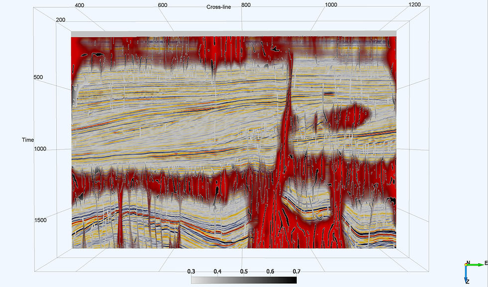
The fault likelihood attribute is a coherency attribute that calculates the possibility of a fault being present on a scale of 0 to 1, where 1 implies a high likelihood of a fault. It is computed on the dip steered median filter cube, for the entire volume of the cube for a selected dip range.

Bigger fault-likelihood (FL) dip computation step-outs help map larger faults by improving their continuity and hence 4-4-100 was selected as the filter size. From the smoothed section, it was evident that there were discontinuities with near vertical dips as the seismic sequences on either side of these discontinuities appeared offset. Hence a smaller dip scan range of 65-89 degrees was selected.

The thinned fault likelihood (TFL) was then computed. This uses the fault likelihood dataset created and creates more linear fault features. The figure below shows the thinned faults as black/ grey lines depending on their thinned fault likelihood (see the scale bar). The red regions are regions with a high fault likelihood. The difference between the broad swaths shown by the FL attribute and the narrow linear features shown by the TFL attribute is evident.

Fault Plane Extraction

Fault planes were extracted from the fault likelihood cube. A small section of the cube was taken from time slice 900-1800 as this region showed up in red in the fault likelihood plot. The minimum fault likelihood to create ‘skins’ was set as 0.67 based on the values in the fault likelihood plot. Skins are not planes, but a mesh of points that can be extracted as a plane by the user. Minimum skin size of 1000 was taken for faster computation.

Once the skins were plotted on the seismic section, small skin sizes were removed as the number of faults plotted was large. One major fault was identified (plotted in red). Numerous smaller faults in the region between crossline 400-600 and below z slice 1500 were extracted as well. Three fault sets were categorised based on skin sizes and were plotted in orange, green and grey in decreasing order of skin size.

Seismic Sequence Analysis

A seismic sequence is a sequence of strata bounded at its top and bottom by unconformities

or their correlative conformities (Mitchum, 1977), identified on a seismic section. Within

each seismic sequence there are depositional packages called systems tracts that are

influenced by both the space available for deposition and the sea level at the time of

deposition. A rise in the sea level causes the shoreline (and hence the facies) to shift landward

and is called a transgression, while a seaward shift of the two is called a regression

(Catuneanu, 2002). OpendTect recognizes 4 systems tracts- Falling Stage Systems Tract

(FSST), Lowstand Systems Tract (LST), Highstand Systems Tract (HST) and Transgressive

Systems Tract (TST).

The study area represents a large fluviodeltaic depositional system showing periods of

transgression and regression. To detect all the stratigraphic horizons and assign them a

depositional time and place them in stratigraphic order OpendTect’s Sequence Stratigraphic

Interpretation System (SSIS) was used. SSIS not only tracks chronostratigraphic horizons but can also create a Wheeler transform for the data. It allows for a systems tract interpretation as

well.

The process begins with creating a SteeringCube from the seismic data. This cube contains

dip values for all the sample locations. The next step was to create a HorizonCube from the

SteeringCube to map the chronostratigraphic units. This is a computationally intensive

process and hence only a subsection of the dataset is used- the regions between two horizons

mapped by the user. These are the upper and lower bounding surfaces of the sigmoid

(henceforth called a seismic package). Z slices between 400 to 1140 were selected for all

inlines and crosslines as it contained a prominent sigmoidal bedding pattern. The

HorizonCube is mapped from a point in the thickest part of the package outwards as shown in

figure.

The chronostratigraphic horizons are mapped from point a to a+n, and then using local dip information obtained from the steering cube it moves onto the next line. To accommodate

diverging horizons, new horizons are created, and for converging horizons, the horizons are

merged. This creates a horizon cube which can then be visualised and interpreted with the

help of a Wheeler transform.

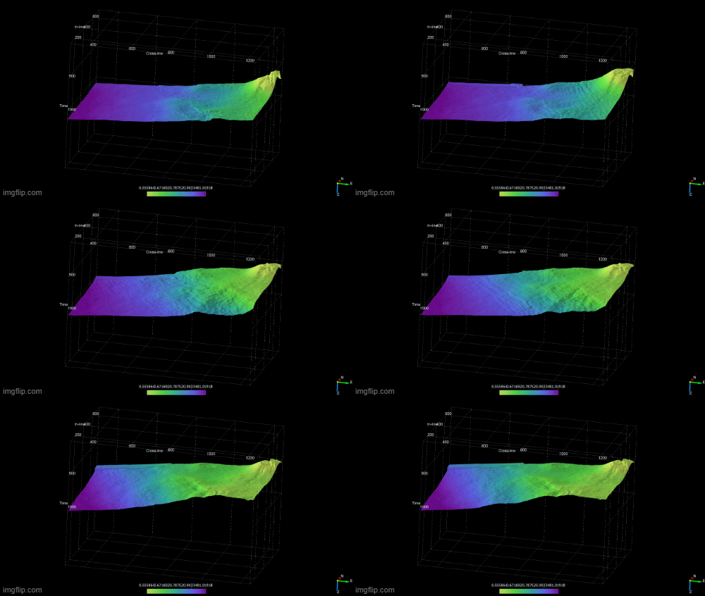
Wheeler transforms (first figure above) are created by flattening each chronostratigraphic event. This enables a clear depiction of periods or erosion or non-deposition in the sequence and gives a clear picture of the lateral extent of a horizon and how it changes with time. Both the Wheeler transform and the mapped chronostratigraphic horizons are viewed simultaneously to identify the systems tracts (second figure above).

The gif below shows the evolution of the delta by creating 3D surfaces for the system tracts.

Salt Dome

Salt domes form when a thick pile of sediments deposits over a large salt bed. The salt being less dense, is forced upwards under the immense pressure of the overlying sediments creating a dome like structure called a salt dome. As the salt rises up, it pushes the overlying sedimentary layers and leads to the formation of radial faults in these layers. Salt domes appear as a very noisy regions or reflection free regions in the seismic data as salt distorts the seismic ray paths. Three methods were used to detect the salt dome in F3.

Thinned Fault Likelihood attribute

The thinned fault likelihood attribute was used to scan the seismic sections for radial fault patterns. Z slice 1500 showed such a pattern. Two other regions showed structures similar to radial faults, but they were very close to a major fault and could be deformation due to smaller fault sets.

Curvature attribute

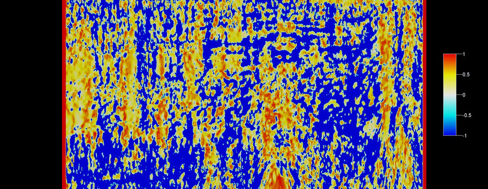
The curvature attribute was used to study inline 690 and crossline 850 as they intersected this pattern. This attribute calculates how much a curve deviates from a straight line. The inline and crossline stepout was set at 10 to increase computation speed and the output was set as Shape Index. The shape index output plots the section on a scale of -1 to 1 describing the surface morphology where -0.5 is a valley, +0.5 is a ridge, 0 is a flat surface and 1 is a dome. The same region identified using the radial fault pattern showed up as a dome.

Polar dip attribute

Inline and crossline dips are converted to true dips. It was calculated on steering cube data using the equation:

Polar dip = √ [(inline dip)2 + (crossline dip)2] μseconds/meters

Regions with high dip values can be interpreted as salt domes, as they deform the strata around them when they push upwards. The same region identified by the previous two methods was seen to have very high dip values.